2. Running the model¶
The command, the examples, what each input file says, a first experiment, and how to read the results.
Note
This chapter assumes ASYNCH is installed (chapter 1). Commands are run from the examples folder.
asynch stands for the program: ../build/src/asynch if you did not run make install, simply asynch inside
Docker.
2.1 The command¶
mpirun -n 4 asynch myrun.gbl
Part of the command |
Meaning |
|---|---|
|
run on 4 processors (MPI processes). 1 is fine for small basins. More than your computer’s cores needs |
|
the program |
|
the global file describing the run. Input and output file names written in it are relative to the folder you are in, not to the |
Options, placed before the .gbl: -m (or --more) prints how long each initialisation step took;
-v prints the version; -h prints the help; -d waits for a key press at start, so a debugger can be attached.
Important
With several processes the results can differ in the last digits from one run to the next (the asynchronous scheduling, chapter 4). With one process a run is exactly repeatable.
2.2 The examples¶
All in examples/. Run times are for one process on a laptop-class computer.
Global file |
Basin, model |
What it shows |
Time |
|---|---|---|---|
|
11 links, model 190 (constant runoff coefficient) |
the smallest complete run; one day, rain for 200 minutes |
1 s |
|
same |
tolerances and solver chosen per link, from |
1 s |
|
same |
the configuration that produced the reference results |
1 s |
|
6 359 links, model 254 (top layer) |
a larger network with the Top Layer model; one day |
4 s |
|
same |
reproduces the reference results |
8 s |
|
11 links, models 192, 196, 258, 259 |
other models; run them from inside their folder ( |
1 s |
Each example has reference results. Chapter 9 explains how they are checked automatically.
2.3 The global file (.gbl), block by block¶
The global file answers a fixed list of questions, in a fixed order. Lines starting with % are
comments, and blank lines are ignored. This is examples/test.gbl, with the meaning of each answer.
The complete reference is docs/input_output.rst (section Global File Structure).
In |
Question |
Notes |
|---|---|---|
|
which model? |
the model number; each needs its own parameters and files ( |
|
start and end (UTC) |
inside ASYNCH, time is counted in minutes since the start |
|
add parameter values to output file names? |
0 = no |
|
what to write in the hydrographs |
|
|
format of the peak-flow file |
always |
|
global parameters: how many, then the values |
same for all links; meaning depends on the model (for 190: v_r, λ₁, λ₂, RC, v_h, v_g) |
|
memory buffers |
keep these values |
|
network (0 = file) |
|
|
link parameters (0 = file) |
|
|
initial state (1 = same for all links) |
0 = |
|
forcings: how many, then one block each |
here rain from a |
|
dams, reservoirs |
0 = none |
|
hydrographs: format, interval [min], file |
1 = |
|
peak flows: format, file |
1 = |
|
which links: for hydrographs (the ids listed in |
|
|
snapshots |
1 = |
|
name for temporary files |
|
|
step-size control (facmin, facmax, safety factor) |
keep these values |
|
tolerances given below (1 = from an |
|
4 lines |
tolerances per state: absolute, relative, absolute and relative for interpolated values |
smaller = more accurate and slower |
2.4 Choosing the numerical solver¶
The numerical solver is the method ASYNCH uses to advance the equations of every link in time. You choose it with
one number in the global file, the number on the line after %Numerical solver index. The documentation calls
this number the solver index: “index 2” simply means “the solver you get when you write 2 there”. There is no
hidden default: every global file states its solver, and all examples use 2.
Write |
Solver |
When to use it |
|---|---|---|
|
Dormand–Prince 5(4) |
the standard choice, used by all examples and by ASYNCH since 2015 |
|
Rodas5P, stiff solver (since 1.7) |
long runs and large networks: usually several times faster at the same accuracy, with more precise peaks. Not for models 21, 22, 23, 40, 261, 262 or a model 255 with dams |
|
RK 3(2), lower order |
tests and teaching; slower for the same accuracy |
|
RK 4(3), lower order |
idem |
Any other number (for example 3) stops the run with a message (2.8).
Why a stiff solver? In a basin some water moves in minutes (a small hillslope) and some in days (the river, the
groundwater). Solvers 0 to 2 must then take very small steps even when nothing is happening. The stiff solver does
not have this limit, so it takes far fewer steps. The details and measurements are in
chapter 4, section 4.7.
Switching from Dormand–Prince (2) to the stiff solver (4)¶
Two changes, both in the %Numerical solver settings block at the end of the global file:
change the solver number from
2to4;divide the four lines of error tolerances by 100 (for example
1e-4becomes1e-6,1e-6becomes1e-8).
Before (Dormand–Prince), in a global file of model 254 (7 states, so 7 numbers per line):
%Solver flag (0 = data below, 1 = .rkd)
0
%Numerical solver index (0 = RK 3(2), 1 = RK 4(3), 2 = Dormand-Prince 5(4), 4 = Rodas5P, stiff)
2
%Error tolerances (abs, rel, abs dense, rel dense)
1e-4 1e-4 1e-4 1e-4 1e-4 1e-4 1e-4
1e-6 1e-6 1e-6 1e-6 1e-4 1e-4 1e-4
1e-4 1e-4 1e-4 1e-4 1e-4 1e-4 1e-4
1e-6 1e-6 1e-6 1e-6 1e-4 1e-4 1e-4
After (stiff solver, tolerances ÷ 100):
%Solver flag (0 = data below, 1 = .rkd)
0
%Numerical solver index (0 = RK 3(2), 1 = RK 4(3), 2 = Dormand-Prince 5(4), 4 = Rodas5P, stiff)
4
%Error tolerances (abs, rel, abs dense, rel dense)
1e-6 1e-6 1e-6 1e-6 1e-6 1e-6 1e-6
1e-8 1e-8 1e-8 1e-8 1e-6 1e-6 1e-6
1e-6 1e-6 1e-6 1e-6 1e-6 1e-6 1e-6
1e-8 1e-8 1e-8 1e-8 1e-6 1e-6 1e-6
Nothing else changes: same input files, same output files, same command. To go back, restore the 2 and the
original tolerances.
Why divide the tolerances by 100?
The tolerances tell a solver how large an error it may make. Dormand–Prince is forced into small steps anyway, so it ends up much more accurate than its tolerances ask. The stiff solver uses the tolerances fully. With the same numbers it is about 16 times faster but its hydrographs differ by up to about 1 % of the peak flow; with tolerances ÷ 100 it is about 6 times faster and as accurate as Dormand–Prince (peaks even more accurate). Measured with model 254 on a 6 359-link network (section 4.7).
Check it on your basin
Speed-ups depend on the model and the basin. Before switching a production setup, run one event with both solvers and compare the hydrographs at your gauges (2.6 shows how to compare two runs).
From Python, the same two changes:
from asynch import GlobalConfig

cfg = GlobalConfig.read("my_basin.gbl")
cfg.solver = 4                                              # stiff solver
for tol in (cfg.abstol, cfg.reltol, cfg.abstol_dense, cfg.reltol_dense):
    tol[:] = [v / 100 for v in tol]                         # tolerances / 100
cfg.write("my_basin_stiff.gbl")                             # run it with asynch, or with Simulation(cfg)
Different solvers on different links. With the solver flag 1, the solver and the tolerances are read from an
.rkd file, one line per link, and the solver number is the last value of each line (docs/input_output.rst,
RK Data Files). This is rarely needed.
2.5 The other input files¶
The small files of the test example can be read by eye. Each starts with the number of links, then one block
per link, starting with its id:
test.rvr · the network
11
1
3 2 8 3
9
0
test.prm · link parameters
11
1
0.4267 0.2622 0.0469
9
0.0896 0.4318 0.0896
test.str · rain
11
1
3
0    40
100  20
200   0
The other files of the example:
File |
Content |
|---|---|
|
12 values: the potential evaporation of each month [mm/month] |
|
the link ids for which hydrographs are written |
|
tolerances and method per link; format in Input/Output Formats (RK Data Files) |
|
the initial state: one value per state, used for every link (below) |
clearcreek.uini · the initial state
254
0.000000

1e-6 0.0 0.0 0.0 0.0 0.0 1e-6
If the file gives fewer values than the model has states, ASYNCH warns and sets the missing ones to 0. For model 254, the last three are always recomputed anyway (chapter 5).
2.6 Exercise: change a parameter and compare¶
The best way to learn the model is to change one thing and look at the effect. Here: the runoff coefficient RC of model 190 (the fraction of rain that runs off; 4th global parameter), from 0.33 to 0.50.
Copy the global file, and create a folder for the new results.
cd examples
cp test.gbl test_rc05.gbl
mkdir -p run_rc05
ASYNCH does not create folders: if one is missing, it stops at once with
Error: cannot write the hydrographs: the folder "run_rc05" does not exist(§2.8).Edit the copy. Open
test_rc05.gblin a text editor (nano test_rc05.gbl, or any editor) and change four lines: the runoff coefficient, and the three output files, which go to the new folder (red: before, green: after).- 6 0.33 0.20 -0.1 0.33 0.1 2.2917e-5 + 6 0.33 0.20 -0.1 0.50 0.1 2.2917e-5 - 5 5.0 outputs.h5 + 5 5.0 run_rc05/outputs.h5 - 1 test.pea + 1 run_rc05/test.pea - 4 60 test.h5 + 4 60 run_rc05/test.h5
Run both, and plot the outlet (link 80).
mpirun -n 2 asynch test.gbl
mpirun -n 2 asynch test_rc05.gbl
python3 ../tools/python/plot_hydrographs.py --link 80 outputs.h5 run_rc05/outputs.h5 \
        --labels "RC = 0.33" "RC = 0.50" --out rc_compare.png
You should see
The peak of each run, and a new file
rc_compare.png(below):RC = 0.33: link 80, maximum 1.93612 at 2.00 h RC = 0.50: link 80, maximum 2.98869 at 1.92 h
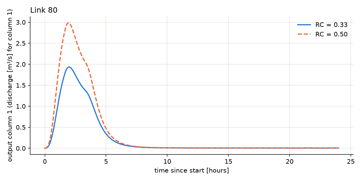
A larger runoff coefficient gives a higher peak (+54 % for +52 % of RC), and the peak comes slightly
earlier: the channel velocity grows with discharge (the exponent λ₁ in the channel equation, chapter 5).
The same recipe works for any change: rain in the .str file, dates, tolerances, or another model.
2.7 Reading the results¶
File |
Content |
|---|---|
|
one line per link: |
|
hydrographs as text: for each saved link, a header |
|
hydrographs for spreadsheets: one group of columns per link |
|
hydrographs as a table with columns |
|
hydrographs as arrays: |
|
all states of all links at one time; can be the initial state of a next run (flags 2 and 4 of the initial-state block) |
.pea, .dat and .csv are text files, and open in any editor or spreadsheet. h5dump -H file.h5 shows the
structure of an .h5 file.
tools/python/asynch_io.py reads every format into dictionaries {link id: array}:
import sys; sys.path.insert(0, "../tools/python")
import asynch_io

h = asynch_io.read_h5_hydrographs("outputs.h5")     # {link: [time, State0]}
print("outlet peak:", h[80][:, 1].max(), "m3/s")

peaks = asynch_io.read_pea("test.pea")              # {link: (area, time of peak, peak)}
print(peaks[80])
and tools/python/plot_hydrographs.py plots one link from up to three files (§2.6). The asynch Python package
reads them too (asynch.io, chapter 10).
2.8 Messages you may see¶
Message |
Meaning, and what to do |
|---|---|
|
the model number in the initial-state file differs from the |
|
fewer initial values than states: the others are 0, or computed by the model. Fine if intended |
|
fix the number after |
|
wrong name or wrong folder: file names are relative to where you run |
|
the file was edited on Windows: convert it with |
|
the rain file does not match the network |
|
ASYNCH checks every output folder before computing: create the folder ( |
|
writing the results failed at the end of the run (disk full, folder deleted, …); |
|
see the format in |
|
more global parameters than the model uses; the extra ones are ignored |